MXNet made simple: Clojure Symbol API

Friday. March 01, 2019 - 12 mins

In a previous post, we explained what NDArrays are and how they are the building blocks of the MXNet framework.

Now it is time to look at the Symbol API that lets us define a Computation Graph.

Before we begin…

We will need to import certain packages:

(require '[org.apache.clojure-mxnet.dtype :as d])
(require '[org.apache.clojure-mxnet.ndarray :as ndarray])
(require '[org.apache.clojure-mxnet.symbol :as sym])

Computation Graph and Symbols

A Neural Network is a description of a computation to perform. Multiply this weight matrix with this input vector, perform an activation function, and so on. MXNet gives us the tools to express these operations as a Graph of Computations.

Below is an example of a simple computation graph. It describes what E is in terms of operations and dependencies.

Example of Computation Graph

Computation Graph: E = (A * B) + (C * D)

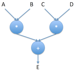
This Graph is a description of the operations that are needed to compute (A * B) + (C * D). At this point, nobody cares what A, B, C or D are. They are pure symbols.

Here is how one can define this computation graph in MXNet

;; Define Input data as Variable
(def a (sym/variable "A"))
(def b (sym/variable "B"))
(def c (sym/variable "C"))
(def d (sym/variable "D"))

;; Define a Computation Graph: e = (a * b) + (c * d)
(def e
  (sym/+
    (sym/* a b)
    (sym/* c d)))

Interessingly, one can query the information of the symbolic graph with the Symbol API

;; What are the dependencies for `e`?
(sym/list-arguments e) ;["A" "B" "C" "D"]

;; What does `e` compute?
(sym/list-outputs e) ;["_plus0_output"]

;; What is the implementation of `e` as a stack of operations?
(sym/list-outputs (sym/get-internals e)) ;["A" "B" "_mul0_output" "C" "D" "_mul1_output" "_plus0_output"]

One can also render the computation graph. It is a good practice to make sure the operations are well connected and we will also explain how to render computation graphs for Neural Networks.

(require '[org.apache.clojure-mxnet.visualization :as viz])

;; Render Computation Graph
(defn render-computation-graph!
  "Render the `sym` and saves it as a pdf file in `path/sym-name.pdf`"
  [{:keys [sym-name sym input-data-shape path]}]
  (let [dot (viz/plot-network
              sym
              input-data-shape
              {:title sym-name
               :node-attrs {:shape "oval" :fixedsize "false"}})]
    (viz/render dot sym-name path)))

;; Render the computation graph `e`
(render-computation-graph!
  {:sym-name "e"
   :sym e
   :input-data-shape {"A" [1] "B" [1] "C" [1] "D" [1]}
   :path "model_render"})

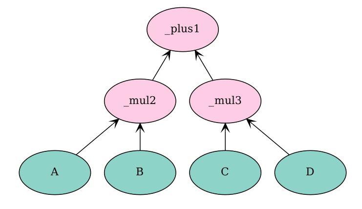
Computation Graph e Rendered with mxnet

Computation Graph: E = (A * B) + (C * D) rendered in MXNet

The two computation graphs are identical. They both describe the same computation E.

Binding NDArrays to Symbols

Now that the computation graph for E is defined, one would like to actually use it to make some calculations. Before being able to run the graph, we need to bind NDArrays to the dependencies of the computation Graph E. In our case, we need to bind NDArrays for A, B, C and D.

Lets bind the following values to the symbols:

A = 1
B = 2
C = 3
D = 4

;; Binding `ndarrays` to `symbols`
(def data-binding
  {"A" (ndarray/array [1] [1] {:dtype d/INT32})
   "B" (ndarray/array [2] [1] {:dtype d/INT32})
   "C" (ndarray/array [3] [1] {:dtype d/INT32})
   "D" (ndarray/array [4] [1] {:dtype d/INT32})})

Now we can run the Graph and get the answer for E

(require '[org.apache.clojure-mxnet.executor :as executor])

;; Execute the graph operations `e`
(-> e
    (sym/bind data-binding)
    executor/forward
    executor/outputs
    first
    ndarray/->vec) ; We got our answer: 1 * 2 + 4 * 3 = 14

You have probably heard that Deep Learning Models need to be trained on GPUs. MXNet gets us covered by letting us choose on which device we want to run the Computation Graph E

(require '[org.apache.clojure-mxnet.context :as context])

;; Execute the graph on a different device (cpu or gpu)
(-> e
    ; (sym/bind (context/cpu 0) data-binding)
    (sym/bind (context/gpu 0) data-binding)
    executor/forward
    executor/outputs
    first
    ndarray/->vec) ; We got our answer: 1 * 2 + 4 * 3 = 14

Serializing Symbols

One can save the computation graph on disk and reload it later to run it with new inputs

(let [symbol-filename "symbol-e.json"]
  ;; Saving to disk symbol `e`
  (sym/save e symbol-filename)
  ;; Loading from disk symbol `e`
  (let [e2 (sym/load symbol-filename)]
    (println (= (sym/to-json e) (sym/to-json e2))) ;true
    ))

Conclusion

This blog post explained the concept of a Computation Graph and how MXNet lets us define them. A Computation Graph can be queried, rendered and run when NDArrays are bound to it. We will use Computation Graphs a lot because Deep Learning Models are Computation Graphs!

Next time, we will learn more about the Module API that allows us to train models and make new predictions.

References and Resources

Here is also the code used in this post - also available in this repository

(ns mxnet-clj-tutorials.symbol
  "Tutorial for the `symbol` API."
  (:require
    [org.apache.clojure-mxnet.context :as context]
    [org.apache.clojure-mxnet.dtype :as d]
    [org.apache.clojure-mxnet.executor :as executor]
    [org.apache.clojure-mxnet.module :as m]
    [org.apache.clojure-mxnet.ndarray :as ndarray]
    [org.apache.clojure-mxnet.symbol :as sym]
    [org.apache.clojure-mxnet.visualization :as viz]))

;;; Composing Symbols

;; Define Input data as Variable
(def a (sym/variable "A"))
(def b (sym/variable "B"))
(def c (sym/variable "C"))
(def d (sym/variable "D"))

;; Define a Computation Graph: e = (a * b) + (c * d)
(def e
  (sym/+
    (sym/* a b)
    (sym/* c d)))

;; What are the dependencies for `e`?
(sym/list-arguments e) ;["A" "B" "C" "D"]

;; What does `e` compute?
(sym/list-outputs e) ;["_plus0_output"]

;; What is the implementation of `e` as a stack of operations?
(sym/list-outputs (sym/get-internals e)) ;["A" "B" "_mul0_output" "C" "D" "_mul1_output" "_plus0_output"]

;; Render Computation Graph
(defn render-computation-graph!
  "Render the `sym` and saves it as a pdf file in `path/sym-name.pdf`"
  [{:keys [sym-name sym input-data-shape path]}]
  (let [dot (viz/plot-network
              sym
              input-data-shape
              {:title sym-name
               :node-attrs {:shape "oval" :fixedsize "false"}})]
    (viz/render dot sym-name path)))

(comment
  ;; Render the computation graph `e`
  (render-computation-graph!
    {:sym-name "e"
     :sym e
     :input-data-shape {"A" [1] "B" [1] "C" [1] "D" [1]}
     :path "model_render"}))

;;; Executing Symbols

;; Binding `ndarrays` to `symbols`
(def data-binding
  {"A" (ndarray/array [1] [1] {:dtype d/INT32})
   "B" (ndarray/array [2] [1] {:dtype d/INT32})
   "C" (ndarray/array [3] [1] {:dtype d/INT32})
   "D" (ndarray/array [4] [1] {:dtype d/INT32})})

;; Execute the graph operations `e`
(-> e
    (sym/bind data-binding)
    executor/forward
    executor/outputs
    first
    ndarray/->vec) ; We got our answer: 1 * 2 + 4 * 3 = 14

;; Execute the graph on a different device (cpu or gpu)
(-> e
    (sym/bind (context/cpu 0) data-binding)
    ; (sym/bind (context/gpu 0) data-binding)
    executor/forward
    executor/outputs
    first
    ndarray/->vec) ; We got our answer: 1 * 2 + 4 * 3 = 14

;;; Serialization - json format

(let [symbol-filename "symbol-e.json"]
  ;; Saving to disk symbol `e`
  (sym/save e symbol-filename)
  ;; Loading from disk symbol `e`
  (let [e2 (sym/load symbol-filename)]
    (println (= (sym/to-json e) (sym/to-json e2))) ;true
    ))

Arthur Caillau

A man who eats parentheses for breakfast